
Github link for MCP Server : https://github.com/shadabshaukat/postgres-mcp-server/
Helping Enterprise DBA's Transition to the Cloud
Github link for MCP Server : https://github.com/shadabshaukat/postgres-mcp-server/
A blue/green deployment works by creating a fully synchronized copy of your production database and running it as a separate staging environment.
In this article I will show how you can build a Blue-Green deployment for your OCI PostgreSQL for doing apps related testing.
Via Logical Replication for Major Version Upgrades or App Performance/Regression Testing
Most DBAs & DevOps people are already familiar with the Blue-Green deployment methodology when deploying a new version of a service. OCI PostgreSQL does not natively support Blue-Green deployment as of when this article was written. But it is quite easy to setup using a few OCI native components and logical replication with pglogical (or OCI Goldengate)
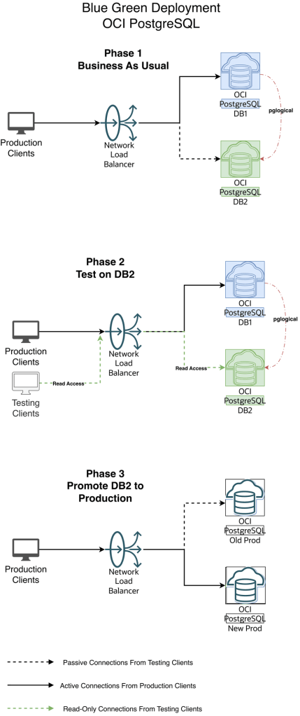
Diagram 1 — Blue-Green Workflow
1.Initial and One time setup:
a. Create an additional new version DB2 OCI PostgreSQL cluster
b. Create OCI DNS Private Zone for the Application for your VCN’s DNS resolver. This Zone will be used by the local applications to connect to OCI PostgreSQL via the OCI Load balancer. If you have an on-premise DNS and need to extend your on-premise DNS to resolve this private zone then refer this documentation : https://docs.oracle.com/en/solutions/oci-best-practices-networking/private-dns-oci-and-premises-or-third-party-cloud.html
c. Create an OCI Network load balancer for their applications to connect to. This LB will act as a proxy to the actual database system.
d. Have the load balancer backend point to the primary endpoint ip address of the database system(say DB1)
2. When we have new changes, do initial load for OCI Postgres between DB1 to DB2 using any of the logical data migration utilities like pg_dump, pg_restore
3. Create publication and subscription from DB1 to DB2 using pglogical (or OCI Goldengate)
4. Have the app tests hit DB2 endpoint to perform read queries, validate and certify the changes
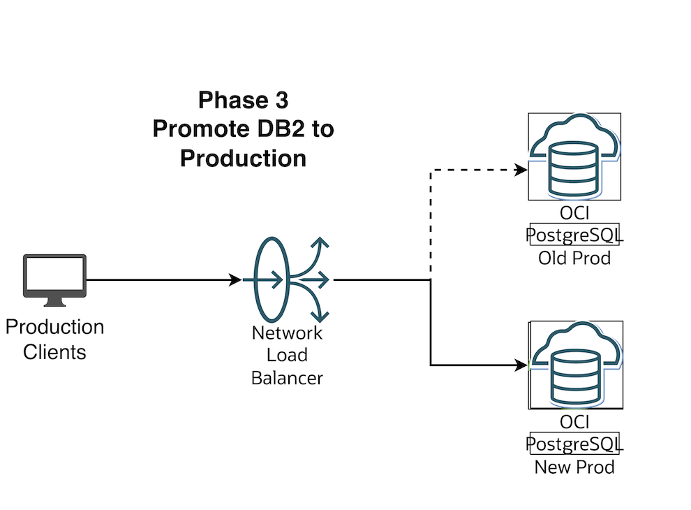
5. When DB2 appears ready for production consumption, orchestrate:
a. Pause any app activity and pause pglogical replication (optional) since pglogical is logical replication tool, the DB2 is always available in Read-Write mode. Just for App testing we are using read-only mode to avoid conflicts and complex scenario of reverse replication from DB2 to DB1
b. Update load balancer backend to the primary endpoint ip address of DB2
c. Stop the replication setup between DB1 and DB2 by stopping the publisher and subscribers
6. Production Client Apps are now connecting to the new Production environment (Green)

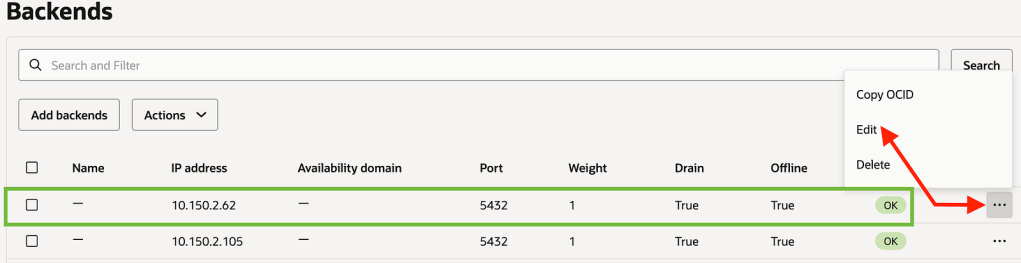
IP : 10.150.2.105
2. OCI PostgreSQL Database v16 which is the Green environment aka Staging

IP : 10.150.2.62
3. OCI Network Load Balancer with the 2 DB endpoints added as backend set fronted with a listener on tcp/5432

Listener

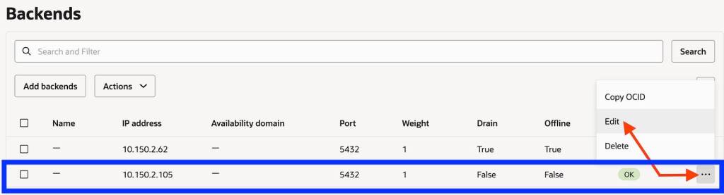
Backends

Make sure the Blue (Production) environment is active and the Green environment backend set is offline and drained.

4. Create an OCI DNS Private zone in your VCN’s DNS resolver
In my case i call my private zone postgres.local
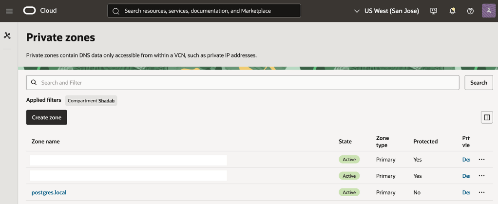

nlb-app.postgres.local is the main FQDN all apps will use to connect the backend database
nlb-app-blue.postgres.local is the FQDN for Blue Database and this is not used by App connections
nlb-app-green.postgres.local is the FQDN for the Green Database and this is used by the App stack which will perform the Read-only queries for validating the application performance.
We will use the OCI Network Load Balancers backend set to make the blue backend IP offline and activate green IP, This incurs a small outage (in seconds depending on TTL of the DNS resolver) where the App moves from connecting to Blue Database to the Final Green Database which is promoted as production.
In this example we are demonstrating using a simple table : https://github.com/shadabshaukat/STAND/blob/main/postgres.sql
################# — Source Blue v15 — #################
Hostname : primary.umiokgnhd4hlpov7xncfwymgxv4pgq.postgresql.us-sanjose-1.oci.oraclecloud.com
Version : 15.12
— Run the following query to grant permissions on the source database to enable logical replication. —
CREATE EXTENSION pglogical;

show oci.admin_enabled_extensions ;
alter role postgres with replication;

grant EXECUTE on FUNCTION pg_catalog.pg_replication_origin_session_reset() to postgres ;

grant EXECUTE on FUNCTION pg_catalog.pg_replication_origin_session_setup to postgres ;

grant all on FUNCTION pg_catalog.pg_replication_origin_session_setup to postgres;
Note : postgres is the admin user created during the database setup process.
— Create the publisher node on the source database. —
SELECT pglogical.create_node(node_name := 'provider1',dsn :='host=primary.umiokgnhd4hlpov7xncfwymgxv4pgq.postgresql.us-sanjose-1.oci.oraclecloud.com port=5432 user=postgres password=RAbbithole1234## dbname=postgres');
node_name: Specify the name of the publisher to be created on the source database.

host: Enter the fully qualified domain name (FQDN) of the source database.

port_number: Provide the port on which the source database is running.

database_name: Specify the database where the publication will be created.
— Include all tables in the public schema to the default replication set. —
SELECT pglogical.replication_set_add_all_tables('default', ARRAY['public']);
replication_set_add_all_tables

 - - - - - - - - - - - - - - - -

 t

(1 row)
################# — Target Green v16 — #################
Hostname : primary.46mtfkxsj6337nqvx2de6gq3a57m4a.postgresql.us-sanjose-1.oci.oraclecloud.com
Version : 16.8
— Run the following query to grant permissions on the target database to enable logical replication. —
CREATE EXTENSION pglogical;

show oci.admin_enabled_extensions ;
alter role postgres with replication;

grant EXECUTE on FUNCTION pg_catalog.pg_replication_origin_session_reset() to postgres ;

grant EXECUTE on FUNCTION pg_catalog.pg_replication_origin_session_setup to postgres ;

grant all on FUNCTION pg_catalog.pg_replication_origin_session_setup to postgres;
Note : postgres is the admin user created during the database setup process.
— Create the subscriber node on target database. —
SELECT pglogical.create_node(node_name := 'subscriber1',dsn :='host=primary.46mtfkxsj6337nqvx2de6gq3a57m4a.postgresql.us-sanjose-1.oci.oraclecloud.com port=5432 user=postgres password=RAbbithole1234## dbname=postgres');
node_name: Define the name of the subscriber on the target database.

host: Enter the fully qualified domain name (FQDN) of the target database.

port_number: Enter the port on which the target database is running.

database_name: Provide the name of the database where the subscription will be created.
— Create the Schema-only on Target Database. This can also be done with pg_dump and pg_restore or psql —
CREATE TABLE orders (

 order_id SERIAL PRIMARY KEY,

 customer_id INTEGER,

 product_id INTEGER,

 product_description VARCHAR(500),

 order_delivery_address VARCHAR(500),

 order_date_taken DATE,

 order_misc_notes VARCHAR(500)

);
CREATE OR REPLACE FUNCTION add_random_orders(n INTEGER) RETURNS TEXT AS $$

DECLARE

 i INTEGER := 1;

 v_customer_id INTEGER;

 v_product_id INTEGER;

 v_product_description VARCHAR(500);

 v_order_delivery_address VARCHAR(500);

 v_order_date_taken DATE;

 v_order_misc_notes VARCHAR(500);

BEGIN

 WHILE i <= n LOOP

 v_customer_id := floor(random() * 100) + 1;

 v_product_id := floor(random() * 50) + 1;

 v_product_description := CONCAT('Product ', floor(random() * 10) + 1);

 v_order_delivery_address := CONCAT('Address ', floor(random() * 10) + 1);

 v_order_date_taken := CURRENT_DATE - (floor(random() * 30) || ' days')::INTERVAL;

 v_order_misc_notes := CONCAT('Note ', floor(random() * 10) + 1);

INSERT INTO orders (customer_id, product_id, product_description, order_delivery_address, order_date_taken, order_misc_notes)

 VALUES (v_customer_id, v_product_id, v_product_description, v_order_delivery_address, v_order_date_taken, v_order_misc_notes);

i := i + 1;

 END LOOP;

RETURN n || ' random orders added.';

EXCEPTION

 WHEN OTHERS THEN

 RAISE EXCEPTION 'Error: %', SQLERRM;

END;

$$ LANGUAGE plpgsql;
— Create the subscription on the subscriber node, which will initiate the background synchronization and replication processes. —
SELECT pglogical.create_subscription(subscription_name := 'subscription1',provider_dsn := 'host=primary.umiokgnhd4hlpov7xncfwymgxv4pgq.postgresql.us-sanjose-1.oci.oraclecloud.com port=5432 user=postgres password=RAbbithole1234## dbname=postgres sslmode=verify-full sslrootcert=/etc/opt/postgresql/ca-bundle.pem');
subscription_name: Provide the name of the subscription.

host: Provide the FQDN of the source database.

port_number: Provide the port on which the target database is running.

database_name: Provide the name of the source database.
Note: Be sure to use sslmode=verify-full and sslrootcert = /etc/opt/postgresql/ca-bundle.pem in subscription creation string to prevent any connection failures.
SELECT pglogical.wait_for_subscription_sync_complete('subscription1');
################# — Target Green v16 — #################
— Run the following statement to check the status of your subscription on your target database. —
select * from pglogical.show_subscription_status();


subscription_name | status | provider_node |

 provider_dsn |

 slot_name | replication_sets | forward_origins

 - - - - - - - - - -+ - - - - - - -+ - - - - - - - -+ - - - - - - - - - - - - - - - - - - - - - - - - - - - - - - - - - - - - - - - - - - -

 - - - - - - - - - - - - - - - - - - - - - - - - - - - - - - - - - - - - - - - - - - - - - - - - - - - - - - - - - - - - - - - - - - - -+

 - - - - - - - - - - - - - - - - - - - + - - - - - - - - - - - - - - - - - - - -+ - - - - - - - - -

 subscription1 | replicating | provider1 | host=primary.umiokgnhd4hlpov7xncfwymgxv4pgq.postgresql.us-sanjose-1.oci.oraclecloud.c

om port=5432 user=postgres password=RAbbithole1234## dbname=postgres sslmode=verify-full sslrootcert=/etc/opt/postgresql/ca-bundle.pem |

 pgl_postgres_provider1_subscription1 | {default,default_insert_only,ddl_sql} | {all}

(1 row)
################# — Source Blue v15 — #################
— Run the following statement to check the status of your replication on your source database. —
SELECT * FROM pg_stat_replication;


pid | usesysid | usename | application_name | client_addr | client_hostname | client_port | backend_start | backend

_xmin | state | sent_lsn | write_lsn | flush_lsn | replay_lsn | write_lag | flush_lag | replay_lag | sync_priority | sync_state |

 reply_time

 - - - -+ - - - - - + - - - - - + - - - - - - - - - + - - - - - - - + - - - - - - - - -+ - - - - - - -+ - - - - - - - - - - - - - - - -+ - - - -

 - - - + - - - - - -+ - - - - - -+ - - - - - -+ - - - - - -+ - - - - - - + - - - - - -+ - - - - - -+ - - - - - - + - - - - - - - -+ - - - - - - + -

 - - - - - - - - - - - - - - -

 18569 | 16387 | postgres | subscription1 | 10.150.2.196 | | 1247 | 2025–12–02 04:50:07.242335+00 |

 | streaming | 0/16BAB50 | 0/16BAB50 | 0/16BAB50 | 0/16BAB50 | | | | 0 | async | 2

025–12–02 05:09:09.626248+00

(1 row)
################# — Target Green v16 — #################
A. Stop or Start the Replication
You can disable the subscription using the following command on your target database.
select pglogical.alter_subscription_disable('subscription_name');
-- Target --

select pglogical.alter_subscription_disable('subscription1');
You can enable the subscription using the following command on your target database.
select pglogical.alter_subscription_enable('subscription_name');
-- Target --

select pglogical.alter_subscription_enable('subscription1');
Note: In subscription_name, enter the name of the subscription created at target.
B. Drop the Subscription
select pglogical.drop_subscription('subscription_name');
-- Target --

select pglogical.drop_subscription('subscription1');
Note: In subscription_name, enter the name of the subscription created at target.
C. Drop the Nodes
To drop the node from your Source or Target database, execute the following command :
select pglogical.drop_node('node_name');

Note: In node_name, enter the node name created in source/target database.
-- Source --

select pglogical.drop_node('provider1');
-- Target --

select pglogical.drop_node('subscriber1');
All the production clients are connected to Blue (Production) DB environment.
NLB has the Blue Environment Active in the Backend Set

We will use psql for the testing. So lets add alias to the App host to make the testing a bit simple.
alias pgblue='PGPASSWORD=YourPasswor@123# psql -h nlb-app-blue.postgres.local -U postgres -d postgres'
alias pggreen='PGPASSWORD=YourPasswor@123# psql -h nlb-app-green.postgres.local -U postgres -d postgres'
alias pgnlb='PGPASSWORD=YourPasswor@123# psql -h nlb-app.postgres.local -U postgres -d postgres'
If we do nslookup on the OCI Network Load Balancer FQDN we can see it resolve to the OCI Network Load Balancer’s IP
$ nslookup nlb-app.postgres.local


Server:  169.254.169.254

Address: 169.254.169.254#53


Non-authoritative answer:

Name: nlb-app.postgres.local

Address: 10.150.2.35
Your Apps are now connecting to the v15 Blue Database via this Endpoint

$ alias | grep pgnlb

alias pgnlb='PGPASSWORD=YourPasswor@123# psql -h nlb-app.postgres.local -U postgres -d postgres'
$ pgnlb


psql (17.7, server 15.12)

SSL connection (protocol: TLSv1.2, cipher: ECDHE-RSA-AES256-GCM-SHA384, compression: off, ALPN: none)

Type "help" for help.
## The Server we're connecting to is the v15.12 which is Blue

Your Testing Apps are now connecting to the v16 Green Database via this Endpoint
$ alias | grep pggreen

alias pggreen='PGPASSWORD=YourPasswor@123# psql -h nlb-app-green.postgres.local -U postgres -d postgres'
$ pggreen

psql (17.7, server 16.8)

SSL connection (protocol: TLSv1.2, cipher: ECDHE-RSA-AES256-GCM-SHA384, compression: off, ALPN: none)

Type "help" for help.
Flip the OCI Network Load Balancer Backend Set (Make sure TTL is as low as possible)
Make the current blue IP backend offline and drain it

Save the changes. In this brief moment there is no connectivity from App to DB and your business users should be notified that there will be a brief outage

If you run pgnlb it will hang as there is no backend IP to connect to
[opc@linux-bastion ~]$ pgnlb
Now let us make the Green environment as online from the backend set and Connect the Apps back.

Save Changes

Now connect with pgnlb
[opc@linux-bastion ~]$ pgnlb

psql (17.7, server 16.8)

SSL connection (protocol: TLSv1.2, cipher: ECDHE-RSA-AES256-GCM-SHA384, compression: off, ALPN: none)

Type "help" for help.
You can see that pgnlb is now connecting to the new upgraded v16 version which is the Green environment
We’ve successfully created a end-to-end Blue-Green Testing Methodolgy for OCI PostgreSQL
Amazon just launched the new Distributed SQ> Aurora Database today.
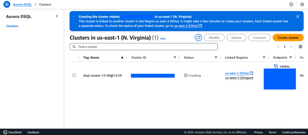
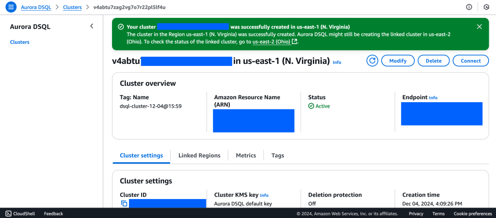
Aurora DSQL is already available as Public Preview in the US Regions. In this article I want to give you the first preview on creating a cluster and connecting to it with psql client.
Go to this link to get started : https://console.aws.amazon.com/dsql/
We will create a Multi-Region with a Linked region and a Witness region.
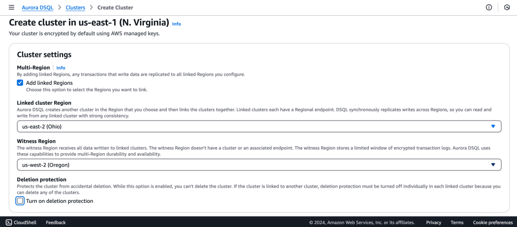
us-east-1 (N Virginia) -> Writer
us-east-2 (Ohio) -> Writer
us-west-2 (Oregon) -> Quorum
https://docs.aws.amazon.com/aurora-dsql/latest/userguide/authentication-token-cli.html
aws dsql generate-db-connect-admin-auth-token \
–expires-in 3600 \
–region us-east-1 \
–hostname <dsql-cluster-endpoint>
The full output will be the password, like below :
v4********4u.dsql.us-east-1.on.aws/?Action=DbConnectAdmin&X-Amz-Algorithm=AWS4-HMAC-SHA256&X-Amz-Credential=AK*****04%2Fus-east-1%2Fdsql%2Faws4_request&X-Amz-Date=202**X-Amz-Expires=3600&X-Amz-SignedHeaders=host&X-Amz-Signature=41e15*****ddfc49
PGSSLMODE=require \
psql –dbname postgres \
–username admin \
–host v4*******u.dsql.us-east-1.on.aws
Password for user admin: <paste-full-string-of-auth-token-output>
psql (17.2, server 16.5)
SSL connection (protocol: TLSv1.3, cipher: TLS_AES_128_GCM_SHA256, compression: off, ALPN: none)
Type “help” for help.
postgres=>
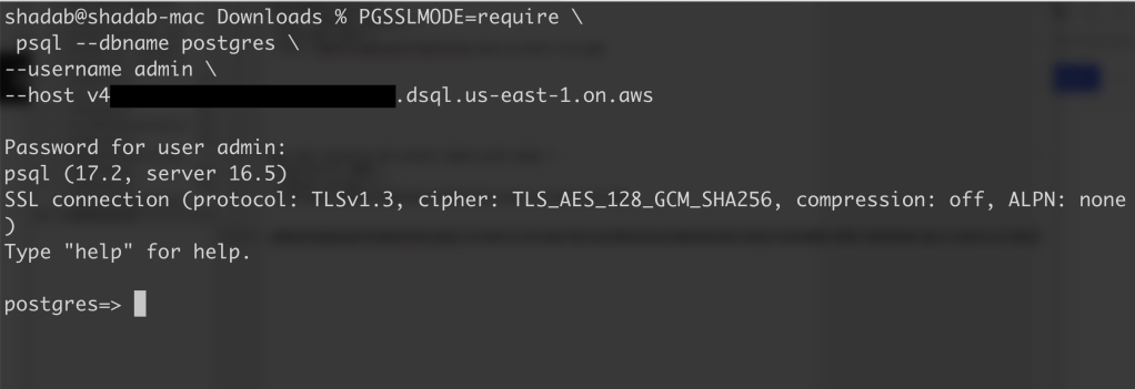
We can connect with a Standard PSQL client!!
CREATE SCHEMA app;
CREATE TABLE app.orders (
order_id UUID PRIMARY KEY DEFAULT gen_random_uuid(),
customer_id INTEGER,
product_id INTEGER,
product_description VARCHAR(500),
order_delivery_address VARCHAR(500),
order_date_taken DATE,
order_misc_notes VARCHAR(500)
);
Sample CSV File to Load Data to Orders Table :
\COPY app.orders (order_id,customer_id,product_id,product_description,order_delivery_address,order_date_taken,order_misc_notes) FROM ‘/Users/shadab/Downloads/sample_orders.csv’ DELIMITER ‘,’ CSV HEADER;
/* Try to wrap the command in a single-line */
[a] Query to Find the Top 5 Customers by Total Orders Within the Last 6 Months
WITH recent_orders AS (
SELECT
customer_id,
product_id,
COUNT(*) AS order_count
FROM
app.orders
WHERE
order_date_taken >= CURRENT_DATE – INTERVAL ‘6 months’
GROUP BY
customer_id, product_id
)
SELECT
customer_id,
SUM(order_count) AS total_orders,
STRING_AGG(DISTINCT product_id::TEXT, ‘, ‘) AS ordered_products
FROM
recent_orders
GROUP BY
customer_id
ORDER BY
total_orders DESC
LIMIT 5;
[b] Query to Find the Most Common Delivery Address Patterns
SELECT
LEFT(order_delivery_address, POSITION(‘,’ IN order_delivery_address) – 1) AS address_prefix,
COUNT(*) AS order_count
FROM
app.orders
GROUP BY
address_prefix
ORDER BY
order_count DESC
LIMIT 10;
[c] Query to Calculate Monthly Order Trends by Product
SELECT
TO_CHAR(order_date_taken, ‘YYYY-MM’) AS order_month,
product_id,
COUNT(*) AS total_orders,
AVG(LENGTH(order_misc_notes)) AS avg_note_length — Example of additional insight
FROM
app.orders
GROUP BY
order_month, product_id
ORDER BY
order_month DESC, total_orders DESC;
You can check latency from AWS Cloud Shell using traceroute to your Aurora DSQL endpoints from different regions
us-east-1 (N Virginia)
$ traceroute v*****u.dsql.us-east-1.on.aws
traceroute to v****u.dsql.us-east-1.on.aws (44.223.172.242), 30 hops max, 60 byte packets
1 * * 216.182.237.241 (216.182.237.241) 1.566 ms
ap-southeast-2 (Sydney)
$ traceroute v*****u.dsql.us-east-1.on.aws
traceroute to v********u.dsql.us-east-1.on.aws (44.223.172.242), 30 hops max, 60 byte packets
1 244.5.0.119 (244.5.0.119) 1.224 ms * 244.5.0.115 (244.5.0.115) 5.922 ms
2 100.65.22.0 (100.65.22.0) 4.048 ms 100.65.23.112 (100.65.23.112) 5.203 ms 100.65.22.224 (100.65.22.224) 3.309 ms
3 100.66.9.110 (100.66.9.110) 25.430 ms 100.66.9.176 (100.66.9.176) 7.950 ms 100.66.9.178 (100.66.9.178) 3.966 ms
4 100.66.10.32 (100.66.10.32) 0.842 ms 100.66.11.36 (100.66.11.36) 2.745 ms 100.66.11.96 (100.66.11.96) 3.638 ms
5 240.1.192.3 (240.1.192.3) 0.263 ms 240.1.192.1 (240.1.192.1) 0.278 ms 240.1.192.3 (240.1.192.3) 0.244 ms
6 240.0.236.32 (240.0.236.32) 197.174 ms 240.0.184.33 (240.0.184.33) 197.206 ms 240.0.236.13 (240.0.236.13) 199.076 ms
7 242.3.84.161 (242.3.84.161) 200.891 ms 242.2.212.161 (242.2.212.161) 202.113 ms 242.2.212.33 (242.2.212.33) 197.571 ms
8 240.0.32.47 (240.0.32.47) 196.768 ms 240.0.52.96 (240.0.52.96) 196.935 ms 240.3.16.65 (240.3.16.65) 197.235 ms
9 242.7.128.1 (242.7.128.1) 234.734 ms 242.2.168.185 (242.2.168.185) 203.477 ms 242.0.208.5 (242.0.208.5) 204.263 ms
10 * 100.66.10.209 (100.66.10.209) 292.168 ms *
References:
[1] Aurora DSQL : https://aws.amazon.com/rds/aurora/dsql/features/
[2] Aurora DSQL User Guide : https://docs.aws.amazon.com/aurora-dsql/latest/userguide/getting-started.html#getting-started-create-cluster
[3] Use the AWS CLI to generate a token in Aurora DSQL : https://docs.aws.amazon.com/aurora-dsql/latest/userguide/authentication-token-cli.html
[4] DSQL Vignette: Aurora DSQL, and A Personal Story : https://brooker.co.za/blog/2024/12/03/aurora-dsql.html
——————————————————————————————–
sudo yum remove awscli

curl "https://awscli.amazonaws.com/awscli-exe-linux-x86_64.zip" -o "awscliv2.zip"

unzip awscliv2.zip

sudo ./aws/install

/usr/local/bin/aws --versionvim ~/.bash_profile
aws --version
aws configure
Create DynamoDB Table

aws dynamodb create-table \
--table-name CustomerRecords \
--attribute-definitions \
AttributeName=CustomerID,AttributeType=S \
AttributeName=RecordDate,AttributeType=S \
--key-schema \
AttributeName=CustomerID,KeyType=HASH \
AttributeName=RecordDate,KeyType=RANGE \
--billing-mode PAY_PER_REQUEST

# Delete DynamoDB Table
aws dynamodb delete-table --table-name CustomerRecords
# Enable Point-in-Time-Recoveryaws dynamodb update-continuous-backups --table-name CustomerRecords --point-in-time-recovery-specification PointInTimeRecoveryEnabled=Trueimport boto3
import faker
import sys
# Generate fake data
def generate_data(size):
fake = faker.Faker()
records = []
for _ in range(size):
record = {
'CustomerID': fake.uuid4(),
'RecordDate': fake.date(),
'Name': fake.name(),
'Age': fake.random_int(min=0, max=100),
'Gender': fake.random_element(elements=('Male', 'Female', 'Other')),
'Address': fake.sentence(),
'Description': fake.sentence(),
'OrderID': fake.uuid4()
}
records.append(record)
return records
def write_data_in_chunks(table_name, data, chunk_size):
dynamodb = boto3.resource('dynamodb')
table = dynamodb.Table(table_name)
for i in range(0, len(data), chunk_size):
with table.batch_writer() as batch:
for record in data[i:i+chunk_size]:
batch.put_item(Item=record)
print(f"Successfully wrote {len(data)} records to {table_name} in chunks of {chunk_size}.")
if __name__ == "__main__":
table_name = 'CustomerRecords'
chunk_size = int(sys.argv[1]) if len(sys.argv) > 1 else 1000
data = generate_data(chunk_size)
write_data_in_chunks(table_name, data, chunk_size)$ python3 load_to_dynamodb.py 1000date +%s
1710374718aws dynamodb export-table-to-point-in-time \
--table-arn arn:aws:dynamodb:ap-southeast-2:11111111:table/CustomerRecords \
--s3-bucket customerrecords-dynamodb \
--s3-prefix exports/ \
--s3-sse-algorithm AES256
--export-time 1710374718aws dynamodb export-table-to-point-in-time \
--table-arn arn:aws:dynamodb:ap-southeast-2:11111111:table/CustomerRecords \
--s3-bucket customerrecords-dynamodb \
--s3-prefix exports_incremental/ \
--incremental-export-specification ExportFromTime=1710374718,ExportToTime=1710375760,ExportViewType=NEW_IMAGE \
--export-type INCREMENTAL_EXPORTImportant Note :
postgres=# SELECT * FROM pg_stat_statements;


postgres=# select * From pg_available_extensions where name ilike 'pg_stat_statements';

        name        | default_version | installed_version |                                comment

--------------------+-----------------+-------------------+--------------------------------------------------------
----------------
 pg_stat_statements | 1.9             |                   | track planning and execution statistics of all SQL stat
ements executed
(1 row)


postgres=# SHOW shared_preload_libraries;

shared_preload_libraries
--------------------------

(1 row)


postgres=# CREATE EXTENSION pg_stat_statements;
CREATE EXTENSION


postgres=# \d pg_stat_statements


postgres=# SELECT *
	 			FROM pg_available_extensions
	 		WHERE
	    		 name = 'pg_stat_statements' and
	   		  installed_version is not null;


        name        | default_version | installed_version |                                comment

--------------------+-----------------+-------------------+--------------------------------------------------------
----------------
 pg_stat_statements | 1.9             | 1.9               | track planning and execution statistics of all SQL stat
ements executed
(1 row)


postgres=# alter system set shared_preload_libraries='pg_stat_statements';
ALTER SYSTEM


postgres=# select * from pg_file_Settings where name='shared_preload_libraries';


                 sourcefile                  | sourceline | seqno |           name           |      setting       |
 applied |            error
---------------------------------------------+------------+-------+--------------------------+--------------------+
---------+------------------------------
 /var/lib/pgsql/14/data/postgresql.auto.conf |          3 |    30 | shared_preload_libraries | pg_stat_statements |
 f       | setting could not be applied
(1 row)


postgres=# exit

##Restart the Instance

sudo systemctl restart postgresql-14

sudo -iu postgres


psql -h localhost -p 5432 -U postgres -d postgres


postgres=# SELECT * FROM pg_stat_statements;

 userid | dbid | toplevel | queryid | query | plans | total_plan_time | min_plan_time | max_plan_time | mean_plan_t
ime | stddev_plan_time | calls | total_exec_time | min_exec_time | max_exec_time | mean_exec_time | stddev_exec_tim
e | rows | shared_blks_hit | shared_blks_read | shared_blks_dirtied | shared_blks_written | local_blks_hit | local_
blks_read | local_blks_dirtied | local_blks_written | temp_blks_read | temp_blks_written | blk_read_time | blk_writ
e_time | wal_records | wal_fpi | wal_bytes
--------+------+----------+---------+-------+-------+-----------------+---------------+---------------+------------
----+------------------+-------+-----------------+---------------+---------------+----------------+----------------
--+------+-----------------+------------------+---------------------+---------------------+----------------+-------
----------+--------------------+--------------------+----------------+-------------------+---------------+---------
-------+-------------+---------+-----------
(0 rows)
PostgreSQL 14 is a powerful and feature-rich open-source relational database management system.
In this guide, we’ll walk through the process of installing and configuring PostgreSQL 14 on Oracle Cloud Infrastructure (OCI) with Oracle Linux 8. The setup includes one master node and two slave nodes, forming a streaming replication setup.
Note : The word slave and replica is used interchangeably in this article when referring to anything which is not a master node
OS– Oracle Linux 8
PostgreSQL Version – 14.10
1 Master Node – IP- 10.180.2.102
2 Slave Nodes – IPs- 10.180.2.152, 10.180.2.58
3 Node PostgreSQL 14 Cluster on OCI

You can create a DR architecture using streaming replication. Put 1 replica in the same region and 2 additional replicas in another OCI region.The VCN’s in both OCI regions have to be remotely peered using a DRG and all routes should permit the traffic over the different subnets and allow communication over port 5432. You can refer to this articleo n how to configure VCN remote peering on OCI: https://docs.oracle.com/en-us/iaas/Content/Network/Tasks/scenario_e.htm
4-Node Cross-Region PostgreSQL 14 Cluster on OCI

Start by updating the system and installing necessary dependencies on both the master and slave nodes:
sudo dnf update -y
sudo dnf module list postgresql
sudo yum -y install gnupg2 wget vim tar zlib openssl
sudo dnf install https://download.postgresql.org/pub/repos/yum/reporpms/EL-8-x86_64/pgdg-redhat-repo-latest.noarch.rpm
sudo yum -qy module disable postgresql
sudo yum install postgresql14-server -y
sudo yum install postgresql14-contrib -y
sudo systemctl enable postgresql-14
sudo postgresql-14-setup initdb
sudo systemctl start postgresql-14
sudo systemctl status postgresql-14
Enable the Postgres user and configure streaming replication on both the master and slave nodes:
sudo -iu postgres
psql -c "ALTER USER postgres WITH PASSWORD 'RAbbithole1234#_';"
tree -L 1 /var/lib/pgsql/14/data
psql -U postgres -c 'SHOW config_file'
              config_file
----------------------------------------
 /var/lib/pgsql/14/data/postgresql.conf
(1 row)
pg_hba.conf and Firewall SettingsUpdate the pg_hba.conf file on both the master and slave nodes to allow connections and adjust firewall settings:
sudo -iu postgres
vim /var/lib/pgsql/14/data/pg_hba.conf
# If ident is available in file then replace 'ident' with 'md5' or 'scram-sha-256'

# Change this line to allow all hosts 0.0.0.0/0

# IPv4 local connections:
host    all             all             0.0.0.0/0               scram-sha-256
exit
sudo systemctl restart postgresql-14
sudo firewall-cmd --list-ports
sudo firewall-cmd --zone=public --permanent --add-port=5432/tcp
sudo firewall-cmd --reload
sudo firewall-cmd --list-ports
On the master node (10.180.2.102), configure streaming replication:
sudo -iu postgres
mkdir -p /var/lib/pgsql/14/data/archive
vim /var/lib/pgsql/14/data/postgresql.conf
## Uncomment and set below parameters
listen_addresses = '*'
archive_mode = on    # enables archiving; off, on, or always
archive_command = 'cp %p /var/lib/pgsql/14/data/archive/%f'
max_wal_senders = 10            # max number of walsender processes
max_replication_slots = 10      # max number of replication slots
wal_keep_size = 50000           # Size of WAL in megabytes; 0 disables
wal_level = replica             # minimal, replica, or logical
wal_log_hints = on               # also do full page writes of non-critical updates

## Only set below if you want to create synchronous replication##
synchronous_commit = remote_apply
synchronous_standby_names = '*'
exit
sudo systemctl restart postgresql-14
netstat -an | grep 5432
Update pg_hba.conf on the master node:
sudo -iu postgres
vim /var/lib/pgsql/14/data/pg_hba.conf
#Add below entry to end of file

host    replication     all             10.180.2.152/32         scram-sha-256
host    replication     all             10.180.2.58/32         scram-sha-256
exit
sudo systemctl restart postgresql-14
On the slave nodes (10.180.2.152 and 10.180.2.58), configure streaming replication:
sudo -iu postgres
mkdir -p /var/lib/pgsql/14/data/backup
vim /var/lib/pgsql/14/data/pg_hba.conf
exit
sudo systemctl restart postgresql-14
sudo chmod 0700 /var/lib/pgsql/14/data/backup
sudo -iu postgres
#Backup and Clone Database from Slave Node using IP of Master Node
pg_basebackup -D /var/lib/pgsql/14/data/backup -X fetch -p 5432 -U postgres -h 10.180.2.102 -R
cd /var/lib/pgsql/14/data/backup
cat postgresql.auto.conf
#Stop the Instance and Restart using Data in New location
/usr/pgsql-14/bin/pg_ctl stop
/usr/pgsql-14/bin/pg_ctl start -D /var/lib/pgsql/14/data/backup
waiting for server to start....2023-11-27 03:36:48.205 GMT [169621] LOG:  redirecting log output to logging collector process
2023-11-27 03:36:48.205 GMT [169621] HINT:  Future log output will appear in directory "log".
 done
server started
Check the status of streaming replication from slave nodes using psql:
psql -h localhost -p 5432 -U postgres -d postgres
postgres# select pg_is_wal_replay_paused();
 pg_is_wal_replay_paused
-------------------------
 f
(1 row)

Note - f means , recovery is running fine. t means it is stopped.
postgres# select * from pg_stat_wal_receiver;
-[ RECORD 1 ]---------+-------------------------------------------------------------------------------------------------------------------------------------------------------------------------------------------------------------------------------------------------------------------------------------
pid                   | 414090
status                | streaming
receive_start_lsn     | 0/A000000
receive_start_tli     | 1
written_lsn           | 0/A002240
flushed_lsn           | 0/A002240
received_tli          | 1
last_msg_send_time    | 2023-12-04 11:40:51.853918+00
last_msg_receipt_time | 2023-12-04 11:40:51.853988+00
latest_end_lsn        | 0/A002240
latest_end_time       | 2023-11-30 08:16:43.217865+00
slot_name             |
sender_host           | 10.180.2.102
sender_port           | 5432
conninfo              | user=postgres password=******** channel_binding=prefer dbname=replication host=10.180.2.102 port=5432 fallback_application_name=walreceiver sslmode=prefer sslcompression=0 sslsni=1 ssl_min_protocol_version=TLSv1.2 gssencmode=prefer krbsrvname=postgres target_session_attrs=any
On the master node, check the status of replication:
psql -h localhost -p 5432 -U postgres -d postgres:
postgres# select * from pg_stat_replication;
-[ RECORD 1 ]----+------------------------------
pid              | 382513
usesysid         | 10
usename          | postgres
application_name | walreceiver
client_addr      | 10.180.2.152
client_hostname  |
client_port      | 47312
backend_start    | 2023-11-30 08:11:42.536364+00
backend_xmin     |
state            | streaming
sent_lsn         | 0/A002240
write_lsn        | 0/A002240
flush_lsn        | 0/A002240
replay_lsn       | 0/A002240
write_lag        |
flush_lag        |
replay_lag       |
sync_priority    | 0
sync_state       | async
reply_time       | 2023-12-04 11:43:12.033364+00

-[ RECORD 2 ]----+------------------------------
pid              | 382514
usesysid         | 10
usename          | postgres
application_name | walreceiver
client_addr      | 10.180.2.58
client_hostname  |
client_port      | 35294
backend_start    | 2023-11-30 08:11:42.542539+00
backend_xmin     |
state            | streaming
sent_lsn         | 0/A002240
write_lsn        | 0/A002240
flush_lsn        | 0/A002240
replay_lsn       | 0/A002240
write_lag        |
flush_lag        |
replay_lag       |
sync_priority    | 0
sync_state       | async
reply_time       | 2023-12-04 11:43:10.113253+00
To restart slave nodes, use the following commands:
/usr/pgsql-14/bin/pg_ctl stop
sudo rm -rf /var/lib/pgsql/14/data/backup/postmaster.pid
/usr/pgsql-14/bin/pg_ctl start -D /var/lib/pgsql/14/data/backup
Follow this comprehensive guide to set up PostgreSQL 14 streaming replication on Oracle Cloud Infrastructure with Oracle Linux 8. Ensure high availability and robust backup capabilities for your PostgreSQL database

Introduction:
Change Data Capture (CDC) is a technique used to track changes in a database, such as inserts, updates, and deletes. In this blog post, we will show you how to implement a custom CDC in PostgreSQL to track changes in your database. By using a custom CDC, you can keep a record of changes in your database and use that information in your applications, such as to provide a history of changes, track auditing information, or trigger updates in other systems
Implementing a Custom CDC in PostgreSQL:
To implement a custom CDC in PostgreSQL, you will need to create a new table to store the change information, create a trigger function that will be executed whenever a change is made in the target table, and create a trigger that will call the trigger function. The trigger function will insert a new row into the change table with the relevant information, such as the old and new values of the record, the time of the change, and any other relevant information.
To demonstrate this, we will show you an example of a custom CDC for a table called “employee”. The change table will be called “employee_cdc” and will contain columns for the timestamp, employee ID, old values, and new values of the employee record. The trigger function will be executed after an update on the “employee” table and will insert a new row into the “employee_cdc” table with the relevant information. Finally, we will show you how to query the “employee_cdc” table to retrieve a list of all changes that have occurred in the “employee” table since a certain timestamp.
CREATE TABLE employee (
id SERIAL PRIMARY KEY,
name VARCHAR(100) NOT NULL,
department VARCHAR(50) NOT NULL,
salary NUMERIC(10,2) NOT NULL,
hire_date DATE NOT NULL
);
CREATE TABLE employee_cdc (
timestamp TIMESTAMP DEFAULT now(),
employee_id INTEGER,
old_values JSONB,
new_values JSONB
);
In this table, “id” is an auto-incremented primary key, “timestamp” is a timestamp with time zone to store the time of the change, “employee_id” is the primary key of the employee record that was changed, and “old_values” and “new_values” are text columns to store the old and new values of the employee record, respectively.
2. Create the Audit table
CREATE TABLE employee_audit (
audit_timestamp TIMESTAMP DEFAULT now(),
employee_id INTEGER,
old_values JSONB,
new_values JSONB
);
3. Create the trigger function
To capture the changes in the employee table, you will need to create a trigger function that will be executed whenever a record is inserted, updated, or deleted in the table. The trigger function will insert a new row into the “employee_cdc” table with the relevant information. Here is an example trigger function:
CREATE OR REPLACE FUNCTION employee_cdc() RETURNS TRIGGER AS $$
BEGIN
IF (TG_OP = 'UPDATE') THEN
INSERT INTO employee_cdc (timestamp, employee_id, old_values, new_values)
VALUES (now(), NEW.id, row_to_json(OLD), row_to_json(NEW));
INSERT INTO employee_audit (employee_id, old_values, new_values)
VALUES (NEW.id, row_to_json(OLD), row_to_json(NEW));
END IF;
RETURN NULL;
END;
$$ LANGUAGE plpgsql;
This trigger function uses the “row_to_json” function to convert the old and new values of the employee record into JSON strings, which are then stored in the “old_values” and “new_values” columns of the “employee_cdc” table. The “NOW()” function is used to get the current timestamp.
4. Create the trigger
Now that the trigger function has been created, you need to create the trigger on the “employee” table that will call the function whenever a record is updated. You can create the trigger with the following command:
CREATE TRIGGER employee_cdc_trigger
AFTER UPDATE ON employee
FOR EACH ROW
EXECUTE FUNCTION employee_cdc();
4. Query the CDC table
In your application code, you can query the “employee_cdc” table to get a list of all changes that have occurred since a certain timestamp. For example, to get all changes since January 1st, 2023, you can use the following SQL query:
SELECT * FROM employee_cdc
WHERE timestamp >= '2023-01-01 00:00:00';
You can then process these changes as needed in your application code.
Conclusion:
In this blog post, we have shown you how to implement a custom Change Data Capture (CDC) in PostgreSQL to track changes in your database. By using a custom CDC, you can keep a record of changes in your database and use that information in your applications. Whether you are tracking changes for auditing purposes, providing a history of changes, or triggering updates in other systems, a custom CDC is a useful tool to have in your PostgreSQL toolkit.
Create DMS Replication From MongoDB 4.2 on EC2 Linux to Redshift
We will create a hub to spoke replication from Mongo DB 4.2 Database to Redshift Schema. MongoDb is installed in the same VPC as Redshift and DMS replication Instance
MongoDB is a NoSQL Datastore where data in inserted and read in JSON format. Internally, a MongoDB document is stored as a binary JSON (BSON) file in a compressed format. Terminology for database, schema and tables in MongoDB is a bit different when compared to relational databases. Here’s how each jargon in MongoDb compares to one in Redshift/PostgreSQL
| MongoDB | Redshift/PostgreSQL |
| Database | Schema |
| Collection | Table |
| Documents | Records/Rows |
MongoDB does not have a a proper structure for a schema and it is is essentially a document store so data can be inserted without defining a proper schema or a structure. This gives MongoDB a lot of flexibility and hence it is the preferred choice for modern applications as you can start development of your application without defining a data model first. It is a schema-less approach to software architecture, which has its own pros and cons.
In our example we will work through the default database in MongoDB called “admin” and create collections(tables) in it and those tables will be replicated to an equivalent schema in Redshift called “admin” which will hold the different tables. We will go about this in 3 stages:
Stage 1 : Create MongoDB on EC2 AMZN Linux, create the collections and connect to MongoDB from your client machine and check the configuration.
Stage 2: Create Redshift Cluster, Aurora PostgreSQL in Private and Public Subnet and Connect to the All Database instances and check.
Stage 3: Create DMS Replication Instance, DMS Replication Endpoints & DMS Replication Tasks.And finally we will check if all data is being replicated by DMS to all the targets.
Architecture : It is a Hub-to-Spoke Architecture with MongoDB Source Being Replicated to Multiple Heterogeneous Targets. However in this Article we will only configure Replication from MongoDB to Redshift.

You can use AWS ‘MongoDB Quick Start’ guide on AWS to deploy MongoDB into a new VPC or deploy into an existing VPC. The guide has two cloud formation templates which can create a new VPC under your account, configure the public & private subnets and launch the EC2 instances with latest version of MongoDB installed. Check this link for the quick deployment options for MongoDB on AWS : https://docs.aws.amazon.com/quickstart/latest/mongodb/step2.html
OR
If you want to install MongoDB manually then you can follow the below procedure :
1. Create Amazon Linux EC2 Instance
2. Add MongoDB Repo and Install MongoDB on AMZN Linux
$ sudo vi /etc/yum.repos.d/mongodb-org-4.0.repo
[mongodb-org-4.0]
name=MongoDB Repository
baseurl=https://repo.mongodb.org/yum/amazon/2013.03/mongodb-org/testing/x86_64/
gpgcheck=1
enabled=1
gpgkey=https://www.mongodb.org/static/pgp/server-4.2.asc
$ sudo yum -y install mongodb-org
$ sudo service mongod start
$ sudo cat /var/log/mongodb/mongod.log
3 . Create Root login
$ mongo localhost/admin
> use admin
> db.createUser( { user:"root", pwd:"root123", roles: [ { role: "root", db: "admin" } ] } )
> exit
4. Modify mongod configuration file /etc/mongod.conf using vi editor
Change below lines from
# network interfaces
net:
port: 27017
bindIp: 127.0.0.1 # Listen to local interface only, comment to listen on all interfaces.
#security:
To
# network interfaces
net:
port: 27017
bindIp: 0.0.0.0 # Listen to local interface only, comment to listen on all interfaces.
security:
authorization: enabled
5. Restart mongod service
$ sudo service mongod restart
Use admin DB as authentication database and ‘root’ user can be used for CDC full load task.
6. For CDC replication, a rmongodb replica needs to be setup and permissions need to be modified/added as below :
Modify mongod.conf using vi editor
$ sudo vi /etc/mongod.conf
replication:
replSetName: rs0
$ sudo service mongod restart
7. Initiate Replica Set for CDC
$ mongo localhost/admin -u root -p
> rs.status()
{
“ok” : 0,
“errmsg” : “no replset config has been received”,
“code” : 94,
“codeName” : “NotYetInitialized”
}
> rs.initiate()
{
“info2” : “no configuration specified. Using a default configuration for the set”,
“me” : “ip-10-0-137-99.ap-southeast-2.compute.internal:27017”,
“ok” : 1
}
rs0:SECONDARY> rs.status()
{
“set” : “rs0”,
“date” : ISODate(“2019-12-31T05:02:22.431Z”),
“myState” : 1,
“term” : NumberLong(1),
“syncingTo” : “”,
“syncSourceHost” : “”,
“syncSourceId” : -1,
“heartbeatIntervalMillis” : NumberLong(2000),
“majorityVoteCount” : 1,
“writeMajorityCount” : 1,
“optimes” : {
“lastCommittedOpTime” : {
“ts” : Timestamp(1577768528, 5),
“t” : NumberLong(1)
},
“lastCommittedWallTime” : ISODate(“2019-12-31T05:02:08.362Z”),
“readConcernMajorityOpTime” : {
“ts” : Timestamp(1577768528, 5),
“t” : NumberLong(1)
},
“readConcernMajorityWallTime” : ISODate(“2019-12-31T05:02:08.362Z”),
“appliedOpTime” : {
“ts” : Timestamp(1577768528, 5),
“t” : NumberLong(1)
},
“durableOpTime” : {
“ts” : Timestamp(1577768528, 5),
“t” : NumberLong(1)
},
“lastAppliedWallTime” : ISODate(“2019-12-31T05:02:08.362Z”),
“lastDurableWallTime” : ISODate(“2019-12-31T05:02:08.362Z”)
},
“lastStableRecoveryTimestamp” : Timestamp(1577768528, 4),
“lastStableCheckpointTimestamp” : Timestamp(1577768528, 4),
“electionCandidateMetrics” : {
“lastElectionReason” : “electionTimeout”,
“lastElectionDate” : ISODate(“2019-12-31T05:02:07.346Z”),
“electionTerm” : NumberLong(1),
“lastCommittedOpTimeAtElection” : {
“ts” : Timestamp(0, 0),
“t” : NumberLong(-1)
},
“lastSeenOpTimeAtElection” : {
“ts” : Timestamp(1577768527, 1),
“t” : NumberLong(-1)
},
“numVotesNeeded” : 1,
“priorityAtElection” : 1,
“electionTimeoutMillis” : NumberLong(10000),
“newTermStartDate” : ISODate(“2019-12-31T05:02:08.354Z”),
“wMajorityWriteAvailabilityDate” : ISODate(“2019-12-31T05:02:08.362Z”)
},
“members” : [
{
“_id” : 0,
“name” : “ip-10-0-137-99.ap-southeast-2.compute.internal:27017”,
“ip” : “10.0.137.99”,
“health” : 1,
“state” : 1,
“stateStr” : “PRIMARY”,
“uptime” : 80,
“optime” : {
“ts” : Timestamp(1577768528, 5),
“t” : NumberLong(1)
},
“optimeDate” : ISODate(“2019-12-31T05:02:08Z”),
“syncingTo” : “”,
“syncSourceHost” : “”,
“syncSourceId” : -1,
“infoMessage” : “could not find member to sync from”,
“electionTime” : Timestamp(1577768527, 2),
“electionDate” : ISODate(“2019-12-31T05:02:07Z”),
“configVersion” : 1,
“self” : true,
“lastHeartbeatMessage” : “”
}
],
“ok” : 1,
“$clusterTime” : {
“clusterTime” : Timestamp(1577768528, 5),
“signature” : {
“hash” : BinData(0,”nDISrR4afyRUVEQVntFkkVpTJKY=”),
“keyId” : NumberLong(“6776464228418060290”)
}
},
“operationTime” : Timestamp(1577768528, 5)
}
rs0:PRIMARY>
8. Make sure security group is open for dms replication group for the port on your EC2 instance where MongoDB is running (Default MongoDB port is 27017)
9. Add a collection (table) with some data to database ‘admin’ in the mongodb installation
> show collections
db.createCollection("accounts", { capped : true, autoIndexId : true, size :

   6142800, max : 10000 } )
db.accounts.insert({"company": "Booth-Wade",

    "location": "5681 Mitchell Heights\nFort Adamstad, UT 8019B",

    "ip_address": "192.168.110.4B",

    "name": "Mark Becker",

    "eid": 27561})


db.accounts.insert({"company": "Myers,  Smith and Turner",

      "location": "USS BenjaminNlinFP0 AA 40236",

      "ip_address": "172.26.254.156",

      "name": "Tyler clark",

      "eid": 87662})


db.accounts.insert({"company": "Bowen-Harris",

      "location": "Tracey Plaza East Katietown,Sc74695",

      "ip_address": "172.28.45.209",

      "name": "Veronica Gomez",

      "eid": 772122})


> db.accounts.find( {} )
— Insert Many —
db.accounts.insertMany(
[
{“company”: “Booth-Wade”,
“location”: “5681 Mitchell Heights\nFort Adamstad, UT 8019B”,
“ip_address”: “192.168.110.4B”,
“name”: “Mark Becker”,
“eid”: 27561},
{“company”: “Myers, Smith and Turner”,
“location”: “USS BenjaminNlinFP0 AA 40236”,
“ip_address”: “172.26.254.156”,
“name”: “Tyler clark”,
“eid”: 87662},
{“company”: “Bowen-Harris”,
“location”: “Tracey Plaza East Katietown,Sc74695”,
“ip_address”: “172.28.45.209”,
“name”: “Veronica Gomez”,
“eid”: 772122}
]);
— Array Insert —
db.accounts.insertMany( [
{
“_id”: “5e037719f45Btodlcdb492464”,
“accounts”: [
{
“company”: “Booth-Wade”,
“location”: “5681 Mitchell Heights\nFort Adamstad, UT 8019B”,
“ip_address”: “192.168.110.4B”,
“name”: “Mark Becker”,
“eid”: 27561
},
{
“company”: “Myers, Smith and Turner”,
“location”: “USS BenjaminNlinFP0 AA 40236”,
“ip_address”: “172.26.254.156”,
“name”: “Tyler clark”,
“eid”: 87662
},
{
“company”: “Bowen-Harris”,
“location”: “Tracey Plaza East Katietown,Sc74695”,
“ip_address”: “172.28.45.209”,
“name”: “Veronica Gomez”,
“eid”: 772122
}
]
}
]);
— Inventory Nested Array Collection —
db.createCollection(“inventory”, { capped : true, autoIndexId : true, size :
6142800, max : 10000 } )
db.createCollection(“inventory_new”, { capped : true, autoIndexId : true, size :
6142800, max : 10000 } )
db.inventory.insertMany( [
{ item: “journal”, instock: [ { warehouse: “A”, qty: 5 }, { warehouse: “C”, qty: 15 } ] },
{ item: “notebook”, instock: [ { warehouse: “C”, qty: 5 } ] },
{ item: “paper”, instock: [ { warehouse: “A”, qty: 60 }, { warehouse: “B”, qty: 15 } ] },
{ item: “planner”, instock: [ { warehouse: “A”, qty: 40 }, { warehouse: “B”, qty: 5 } ] },
{ item: “postcard”, instock: [ { warehouse: “B”, qty: 15 }, { warehouse: “C”, qty: 35 } ] }
]);
db.inventory_new.insertMany([
{ item: “journal”, qty: 25, tags: [“blank”, “red”], size: { h: 14, w: 21, uom: “cm” } },
{ item: “mat”, qty: 85, tags: [“gray”], size: { h: 27.9, w: 35.5, uom: “cm” } },
{ item: “mousepad”, qty: 25, tags: [“gel”, “blue”], size: { h: 19, w: 22.85, uom: “cm” } }
])
> db.inventory.find( {} )
> show collections
accounts
inventory
inventory_new
system.keys
system.users
system.version
We have created 3 user collections called ‘accounts’,’inventory’ & ‘inventory_new’. These 3 collections(tables) shall be replicated to our targets. Connect and Check from MongoDB Compass on your Client Machine
Create a VPC with Public and Private Subnets. In a real world production scenario, it is always recommended to put your databases in a Private subnet
1. Create Public and Private Subnet
2. Install Redshift in Public Subnet
3. Install Redshift in Private Subnet
If you have different scenario’s of your DMS replication in one VPC and Databases in other VPC or Replicating from on-premise to AWS VPC then you can refer this link : https://docs.aws.amazon.com/dms/latest/userguide/CHAP_ReplicationInstance.VPC.html
Steps : Create Replication Instance > Create Endpoints > Create DMS Tasks
1. Create Replication instance
Go to AWS Console > Database Migration Service > Replication Instance > Create Replication Instance
2. Create Replication Endpoints
a) MongoDB Replication Endpoint
Go to DMS Console > Endpoints > Create Endpoint. Use this link for configuration for your endpoint > https://docs.aws.amazon.com/dms/latest/userguide/CHAP_Source.MongoDB.html
In MongoDB as source you have 2 modes available : Document Mode and Table Mode. Some important points to note in this regard are :
MongoDB is officially supported on versions 2.6.x and 3.x as a database source only. But I have tested it with MongoDB 4.2, which is the latest community version and it works without any issues, However I would advise to stick with the officially certified versions. AWS DMS supports two migration modes when using MongoDB as a source. You specify the migration mode using the Metadata mode parameter using the AWS Management Console or the extra connection attribute nestingLevel when you create the MongoDB endpoint.
Document mode
In document mode, the MongoDB document is migrated as is, meaning that the document data is consolidated into a single column named _doc in a target table.
Table mode
In table mode, AWS DMS transforms each top-level field in a MongoDB document into a column in the target table. If a field is nested, AWS DMS flattens the nested values into a single column. AWS DMS then adds a key field and data types to the target table’s column set.
Connection Attributes
nestingLevel
Value : NONE
ONE
Description : NONE – Specify NONE to use document mode. Specify ONE to use table mode.
extractDocID
Value :true
false
Description : false – Use this attribute when nestingLevel is set to NONE.
Test the Endpoint
b) Create Redshift Replication Endpoint
Test Redshift Endpoint
Once you create the endpoint for Redshift it will automatically adds a DMS endpoint roles and assigns it to the Redshift role. Further down when we create S3 as target endpoint we need to add the S3 permissions via a managed policy to this same role
dms-access-for-endpoint : arn:aws:iam::775867435088:role/dms-access-for-endpoint
c) Create MongoDB-Redshift Database Migration Task
Go to DMS Console > Conversion & Migration > Database Migrations Tasks > Create Task
Before moving ahead step that the security group of Redshift allows ingress rules for port 5439 for 0.0.0.0/0 or preferably the Security Group ID of your Replication Instance is added to the ingress rules for Redshift SG over port 5439. Check this link for more information : https://docs.aws.amazon.com/dms/latest/userguide/CHAP_Target.Redshift.html
In our case DMS Replication Instance SGID is ‘sg-0a695ef98b6e39963’. So SG of Redshift looks like below:
Refer this documentation for more complex VPC setup, It is beyond the scope of this article : https://docs.aws.amazon.com/dms/latest/userguide/CHAP_ReplicationInstance.VPC.html
Checking from Redshift..we can see all the 3 tables from mongodb ‘accounts’,’inventory’ & ‘inventory_new’ are created and also the schema ‘admin’ is automatically created by DMS.
Query all the tables to confirm data is replicated
testdb=# select * from admin.accounts;
_id | array_accounts
——————————————————————————————————-
5e037719f45Btodlcdb492464 | [ { “company” : “Booth-Wade”, “location” : “5681 Mitchell Heights\nFort Adamstad, UT 8019B”, “ip
_address” : “192.168.110.4B”, “name” : “Mark Becker”, “eid” : 27561.0 }, { “company” : “Myers, Smith and Turner”, “location”
: “USS BenjaminNlinFP0 AA 40236”, “ip_address” : “172.26.254.156”, “name” : “Tyler clark”, “eid” : 87662.0 }, { “company” : “B
owen-Harris”, “location” : “Tracey Plaza East Katietown,Sc74695”, “ip_address” : “172.28.45.209”, “name” : “Veronica Gomez”, “
eid” : 772122.0 } ]
9772sjs19f45Btodlcdbk49fk4 | [ { “company” : “Trust Co”, “location” : “Zetland Inc.”, “ip_address” : “12.168.210.2B”, “name”
: “Mert Cliff”, “eid” : 4343.0 }, { “company” : “Mist Ltd.”, “location” : “Cliffstone yard”, “ip_address” : “72.32.254.156”, “
name” : “Kris Loff”, “eid” : 76343.0 }, { “company” : “Coles Supermarket”, “location” : “Randwich St”, “ip_address” : “22.28.4
5.110″, “name” : “Will Markbaeur”, “eid” : 13455.0 } ]
(2 rows)
testdb=# select * from admin.inventory;
oid__id | item | array_instock
————————–+———-+——————————————————————————
5e0bd854fd4602c4b6926d68 | journal | [ { “warehouse” : “A”, “qty” : 5.0 }, { “warehouse” : “C”, “qty” : 15.0 } ]
5e0bd854fd4602c4b6926d69 | notebook | [ { “warehouse” : “C”, “qty” : 5.0 } ]
5e0bd854fd4602c4b6926d6a | paper | [ { “warehouse” : “A”, “qty” : 60.0 }, { “warehouse” : “B”, “qty” : 15.0 } ]
5e0bd854fd4602c4b6926d6b | planner | [ { “warehouse” : “A”, “qty” : 40.0 }, { “warehouse” : “B”, “qty” : 5.0 } ]
5e0bd854fd4602c4b6926d6c | postcard | [ { “warehouse” : “B”, “qty” : 15.0 }, { “warehouse” : “C”, “qty” : 35.0 } ]
(5 rows)
testdb=# select * from admin.inventory_new;
oid__id | item | qty | array_tags | size.h | size.w | size.uom
————————–+———-+—–+——————–+——–+——–+———-
5e0bef1775d0b39f2ef66923 | journal | 25 | [ “blank”, “red” ] | 14 | 21 | cm
5e0bef1775d0b39f2ef66924 | mat | 85 | [ “gray” ] | 27.9 | 35.5 | cm
5e0bef1775d0b39f2ef66925 | mousepad | 25 | [ “gel”, “blue” ] | 19 | 22.85 | cm
(3 rows)
mkdir -p $HOME/docker/persistent_volumes/postgresql
docker pull postgres
docker run --name pg-docker -e POSTGRES_PASSWORD=docker -d -p 5432:5432 -v $HOME/docker/persistent_volumes/postgresql:/var/lib/postgresql/data postgres
docker exec -it pg-docker psql -h localhost -U postgres -d postgres
docker container list
docker stop pg-docker
With Redshift Spectrum, you are billed at $5 per terabyte of data scanned, rounded up to the next megabyte, with a 10 megabyte minimum per query. For example, if you scan 10 gigabytes of data, you will be charged $0.05. If you scan 1 terabyte of data, you will be charged $5.
To find how much data is being transferred by Redshift spectrum queries you will have to look at system table ‘SVL_S3QUERY_SUMMARY’ and a specific field called ‘s3_scanned_bytes’ (number of bytes scanned from Amazon S3). The cost of a Redshift Spectrum query is reflected in the amount of data scanned from Amazon S3.
s3_scanned_bytes – The number of bytes scanned from Amazon S3 and sent to the Redshift Spectrum layer, based on compressed data.
For eg: You can run the below query to determine number of bytes transferred by 1 particular spectrum query
— select s3_scanned_bytes from svl_s3query_summary where query= ;
To determine sum of bytes of all queries from Redshift spectrum
— select sum(s3_scanned_bytes) from svl_s3query_summary ;
To determine sum of bytes of all queries in last one day from Redshift spectrum
— select sum(s3_scanned_bytes) from svl_s3query_summary where starttime >= – interval ’24 hours’;
621900000000
(1 row)
Let’s say we have the figure like the above for one day of spectrum use, then using the Redshift spectrum pricing of $5 per terabyte of data scanned, rounded up to the next megabyte, with a 10 megabyte minimum per query. So we can calculate the cost for one day like below,
621900000000 bytes = 621900000000/1024 = 607324218.75 kilobytes
607324218.75 kilobytes = 607324218.75/1024 = 593090.057373046875 megabytes
593090.057373046875 megabytes = 593090.057373046875 /1024 = 579.189509153366089 gigabytes
579.189509153366089 gigabytes = 579.189509153366089/1024 = 0.565614755032584 terabytes
In this case you will be charged for 0.5657 terabytes.(since it is rounded to the next megabyte) $5*0.5657= 2.83$
So 2.83$ is what you will pay for scanning 0.5657 terabytes of data daily from S3 via Spectrum.
Though there is no SQL query to calculate cost, I have created one to easily summarize the approximate cost of data scanned by loading the bytes value into a cost table and running below SQL:
— create table test_cost (s3_scanned_bytes float8 ) ;
— insert into test_cost values (621900000000);
— select sum(s3_scanned_bytes/1024/1024/1024/1024) s3_scanned_tb, 5*sum(s3_scanned_bytes/1024/1024/1024/1024) cost_in_usd from test_cost ;
s3_scanned_tb | cost_in_usd
——————-+————————————————-
0.565614755032584 | 2.82807377516292
(1 row)
— select round(sum(s3_scanned_bytes/1024/1024/1024/1024),4) s3_scanned_tb, round(5*sum(s3_scanned_bytes/1024/1024/1024/1024),2) cost_in_usd from test_cost ;
s3_scanned_tb | cost_in_usd
——————-+————————————————-
0.5656 | 2.83
(1 row)
This is the easiest way to find the data transferred through Spectrum and the cost associated with it.
P.S: The system table is rotated so it is better calculate per day and store it in another table, if you need to maintain record of the bytes transferred via Spectrum.
[1] Amazon Redshift pricing – https://aws.amazon.com/redshift/pricing/#Redshift_Spectrum_Pricing
[2] Monitoring Metrics in Amazon Redshift Spectrum – https://docs.aws.amazon.com/redshift/latest/dg/c-spectrum-metrics.html
[3] SVL_S3QUERY_SUMMARY – https://docs.aws.amazon.com/redshift/latest/dg/r_SVL_S3QUERY_SUMMARY.html
